Chaos to Curve - How the Central Limit Theorem Tames Wild Distributions

Posted Jan 1, 2025 Updated Jan 17, 2026

By Karthick Raja

14 min read

Introduction

The Central Limit Theorem (CLT) is arguably the most important pillar of modern statistics. It provides the theoretical justification for why we can use the Normal distribution to make inferences about population means, even when the population itself is anything but normal.

This holds true regardless of the shape of the source population distribution, provided the variance is finite. Mathematically, as the sample size $n$ approaches infinity ($n \to \infty$):

\[\bar{X}_n \sim N\left(\mu, \frac{\sigma^2}{n}\right)\]

In simpler terms, as you increase the size of your samples, the “map” of those sample means will always start to look like a bell curve.

This has huge applications in the field of Data science and AI. It enables us to bridge the chaotic world of raw data to structured, predictable world of guassian statistics. Some of the applications of CLT include

Hypothesis testing , AB testing
Normality assumption in Regression models, Log power transformations
Weight initializations, Batch normalization in Deep learning
Monte carlo simulations

In this blog, we will try to take different distributions and see if they follow CLT and see if there any distribution which doesn’t adhere to CLT.

Experimental Setup: Commonly used Distributions and their Parameters

To empirically test the CLT, we analyze several probability distributions. Each distribution represents a different “starting shape” for our population. By varying the parameters and increasing the sample size , we can observe how quickly (or if) the sample means converge to normality.

Distribution	Parameters Used	Description
Binomial	$n=10, p=0.5$	Discrete distribution representing successes in independent trials.
Poisson	$\lambda = 4$	Expresses the probability of a given number of events occurring in a fixed interval.
Uniform	$a=0, b=1$	All outcomes are equally likely within a defined range.
Exponential	$\beta = 1.0$	Describes the time between events in a Poisson process; highly skewed.
Gamma	$k=2, \theta=2$	A flexible, skewed distribution used for waiting times.
Beta	$\alpha=2, \beta=5$	Defined on the interval [0, 1]; can be symmetric or skewed.
Cauchy	$x_0=0, \gamma=1$	A “pathological” distribution with heavy tails and no defined mean/variance.

How to measure normality: Histogram, Boxplot, QQ Plot and statistical tests

Whether the distribution of a sample statistic is Normal or not, depends primarily on three things :

The nature of the original population distribution, like Poisson in the given example
The nature of the sample statistic, like mean and IQR in the given example below
The sample size n, which is 12 in the given example. Larger the nn better one gets the idea about the distribution of the statistic, but it has nothing to do with Normal approximation per say. Here we start from smaller value of nn and go larger till we achieve normal distribution

To see whether these sample statistics have Normal distribution, we are employing three simple graphical techniques namely the histogram, box and whiskers plot and Normal Probability Plot (NPP). For Normal distribution the histogram should be bell shaped, the box and whiskers plot should be symmetric about the central line within the box, and the NPP should be a straight line. Thus we see that though the distribution of the sample mean of Poisson(25) is approximately Normal, that of the sample IQR is not, for n=25.

Example of poisson distribution: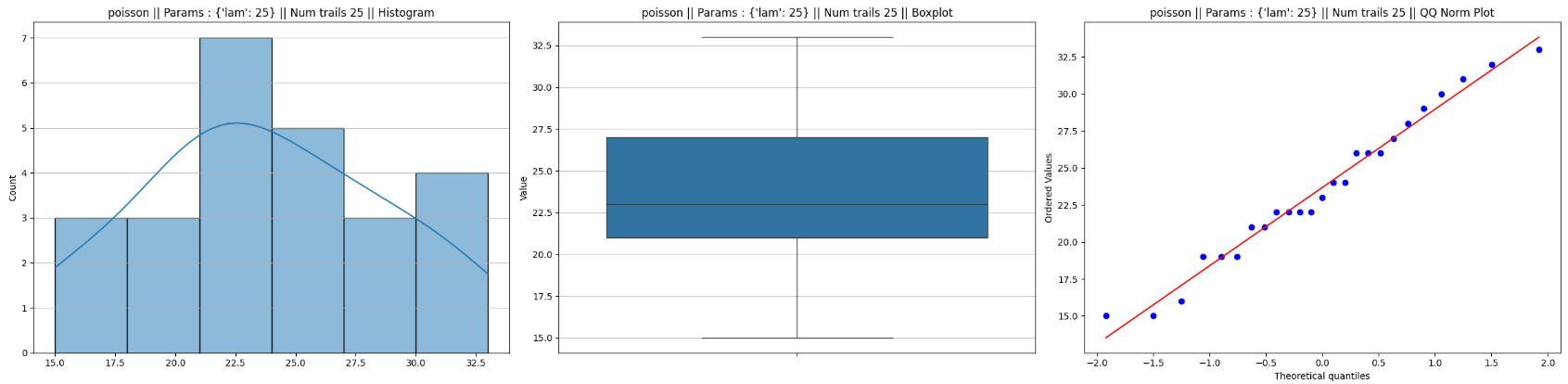

Histogram

The histogram provides a visual representation of the data’s density.

For a Normal Distribution: It should appear symmetric and “bell-shaped.” As increases, the spread (standard error) should narrow around the population mean.

Boxplot

The boxplot summarizes the distribution through quartiles.

For a Normal Distribution: The median should be exactly in the center of the box, and the “whiskers” should be of roughly equal length with very few, if any, outliers.

Quantile-Quantile (QQ) Plot

The QQ plot compares the quantiles of our sample data against the theoretical quantiles of a standard normal distribution.

For a Normal Distribution: The data points should fall along a straight 45-degree diagonal line. Deviations at the ends of the line indicate “heavy tails” or skewness that the CLT hasn’t yet smoothed out.

Python code to generate the above graphs

  
import matplotlib.pyplot as plt
import seaborn as sns
from scipy import stats

def plot_distributions_combined(data_array, title_prefix=''):
    """
    Draws a histogram, boxplot, and QQ norm plot for the input array
    in a single figure with three subplots.

    Args:
        data_array (numpy.ndarray or list): The input data array.
        title_prefix (str): Prefix for the subplot titles.
    """
    fig, axes = plt.subplots(1, 3, figsize=(24, 6))

    # Histogram
    sns.histplot(data_array, kde=True, bins='auto', ax=axes[0])
    axes[0].set_title(f'{title_prefix} Histogram')
    axes[0].grid(axis='y', alpha=0.75)

    # Boxplot
    sns.boxplot(y=data_array, ax=axes[1])
    axes[1].set_title(f'{title_prefix} Boxplot')
    axes[1].set_ylabel('Value')
    axes[1].grid(axis='y', alpha=0.75)

    # QQ Norm Plot
    stats.probplot(data_array, dist="norm", plot=axes[2])
    axes[2].set_title(f'{title_prefix} QQ Norm Plot')

    plt.tight_layout()
    plt.show()

    return fig

Statistical tests for nomality :

Rather than relying soley on visual inspection of histograms or QQ plots, these tests quantify the likelihood that your sample means are drawn from a guassian distribution. The Shapiro-Wilk test is highly sensitive and typically preferred for smaller sample sizes, whereas D’Agostino’s K-squared test focuses on the “shape” of the distribution by measuring its skewness and kurtosis. Using these tests in tandem provides a comprehensive statistical verification.

The Null Hypothesis ($H_0$)In the context of normality testing (for these 2 tests), the Null Hypothesis ($H_0$) is defined as:

$H_0$: The data is sampled from a population that follows a normal distribution.

Interpreting the Results

If $p > 0.05$: We fail to reject the null hypothesis. There is no significant evidence to suggest the data is non-normal (i.e., we assume it is normally distributed)
If $p < 0.05$: We reject the null hypothesis. There is statistically significant evidence that the data does not follow a normal distribution

Python code to check for normality

  
from scipy import stats
import numpy as np

def check_normality(data):
    """
    Performs Shapiro-Wilk, D'Agostino's K-squared, and Anderson-Darling tests for normality.

    Args:
        data (list or array): The numerical data to test.

    Returns:
        dict: A dictionary containing test names as keys and tuples of (statistic, p-value or critical values) as values.
    """
    results = {}

    # Shapiro-Wilk Test
    shapiro_stat, shapiro_p = stats.shapiro(data)
    results['Shapiro-Wilk'] = (shapiro_stat, shapiro_p)

    # D'Agostino's K-squared Test
    dagostino_stat, dagostino_p = stats.normaltest(data)
    results['D_Agostinos_K_squared'] = (dagostino_stat, dagostino_p)

    comment = ""
    if (shapiro_p < 0.05) or (dagostino_p < 0.05):
        comment = "The data is not normally distributed."
    else:
        comment = "The data is normally distributed."

    return results, comment

How to run the simulation ?

We can make use of the existing distribution samplers available in Numpy. These functions draws random samples from a several statistical distribution which models different processes.

Below is the python function for using different numpy functions with several parameters.

  
import numpy as np


def generate_distribution(distribution, params):
    """
    Samples m values from a binomial distribution.

    Args:
        distribution and params
    """

    samples = distribution(**params)
    return samples


def run_trails(distribution, params, n_trails):
  ls_mean = []
  ls_std = []
  for i in range(n_trails):
    samples = generate_distribution(distribution, params)
    mean = np.mean(samples)
    std = np.std(samples)
    ls_mean.append(mean)
    ls_std.append(std)
  return ls_mean, ls_std
  
tests_ = [
    {'binomial': [np.random.binomial, {'n' :12, 'p':0.1}, 50],},
	{'poisson': [np.random.poisson, {'lam':0.001,}, 20],},
	{'uniform': [np.random.uniform, {'low':0, 'high':1,} ,2]},
	{'exponential': [np.random.exponential, {'scale':0.001,}, 10],},
	{'beta': [np.random.beta, {'a':2, 'b':2}, 40],},
	{'gamma': [np.random.gamma, {'shape':0.1, 'scale':1, }, 50],},
	{'cauchy': [np.random.standard_cauchy, {'size':10}, 1000],},
]

ls_figs = []
ls_mean =[]
ls_std = []
for test in tests_:
  for distribution, params in test.items():
    ls_mean, ls_std = run_trails(*params)
    fig = plot_distributions_combined(ls_mean, f"{distribution} || Params : {params[1]} || Num trails {params[2]} ||")
    ls_figs.append(fig)
    test_result , comment = check_normality(ls_mean)
    print(comment)

Results and Discussion

Binomial distribution

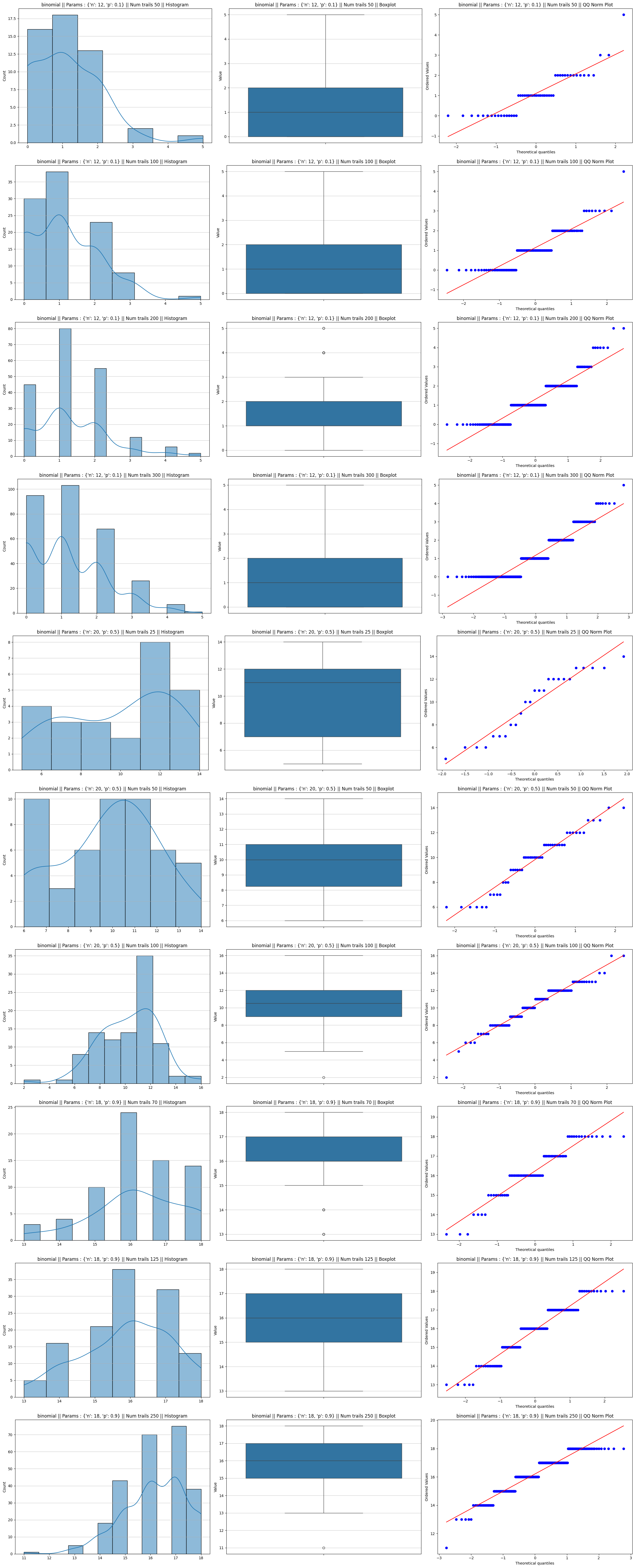
For a Binomial distribution, the shape is determined by the probability $p$ (which you referred to as $\mu$):

When $p = 0.5$: The distribution is perfectly symmetric from the start. Because it doesn’t have to “overcome” any initial skewness, the sample means converge to a Normal distribution very rapidly, often appearing Gaussian with as few as 20 to 25 trials
When $p \to 0$ or $p \to 1$: The distribution becomes heavily skewed (leaning toward one side). For example, if $p = 0.05$, the distribution is mostly zeros with occasional ones. To “smooth out” this extreme lopsidedness into a symmetric bell curve, the CLT requires a much larger sample size $n$

we often use the Success-Failure Condition to determine if a Binomial distribution is “Normal enough” to use Gaussian approximations. We consider it approximately normal only if:

$np \ge 10$
$n(1-p) \ge 10$

As you can see from this rule, if $p = 0.1$, you would need $n \ge 100$ to satisfy the condition, whereas if $p = 0.5$, you only need $n \ge 20$.

Binomial distribution plots

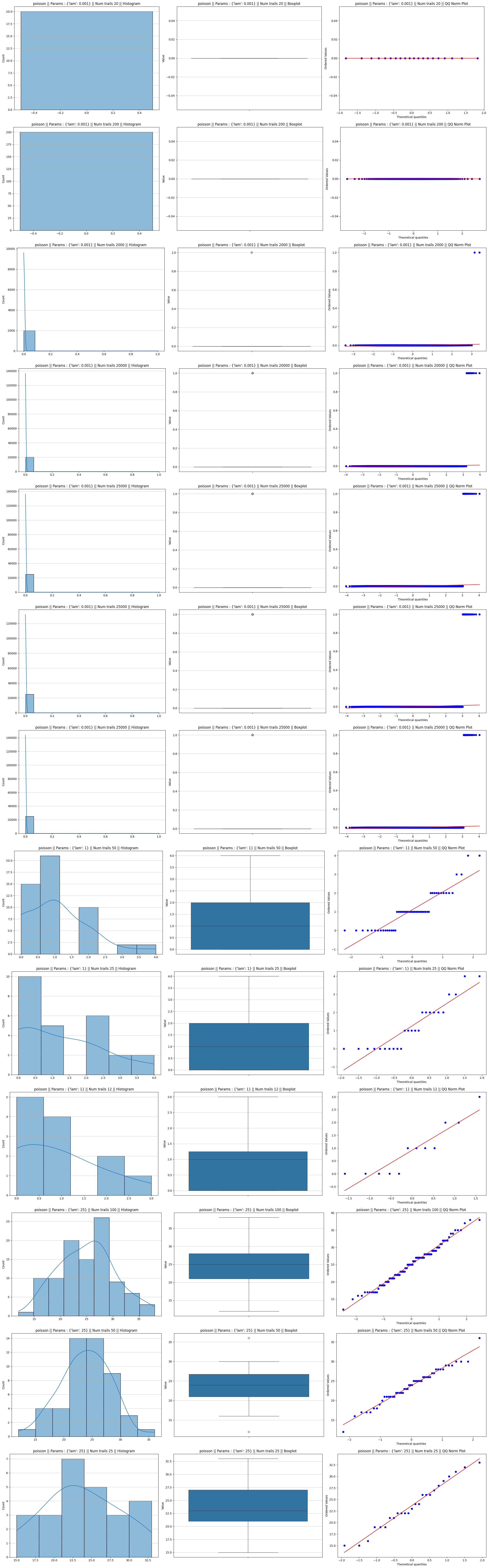
Poisson distribution

In a Poisson distribution, both the mean and the variance are equal to 1$\lambda$.2 The skewness of a Poisson distribution is calculated as:$\text{Skewness} = \frac{1}{\sqrt{\lambda}}$

High $\lambda$ (e.g., 25): The skewness is small ($\frac{1}{\sqrt{25}} = 0.2$). The distribution is already “pre-warmed” to look somewhat symmetric. Consequently, when you take even a modest sample size like $n=50$, the CLT easily pushes the distribution of the mean into a near-perfect Gaussian shape
Low $\lambda$ (e.g., 0.001): The skewness is massive ($\frac{1}{\sqrt{0.001}} \approx 31.6$). At this level, the distribution is almost entirely composed of zeros, with a rare “1” appearing once in a blue moon. It looks more like a vertical line than a curve. To “balance out” these rare events and create the characteristic tails of a Normal distribution, you need thousands of samples ($n > 2000$) to satisfy the theorem

the “speed” of convergence depends on the initial symmetry of the source distribution

Poisson distribution plots

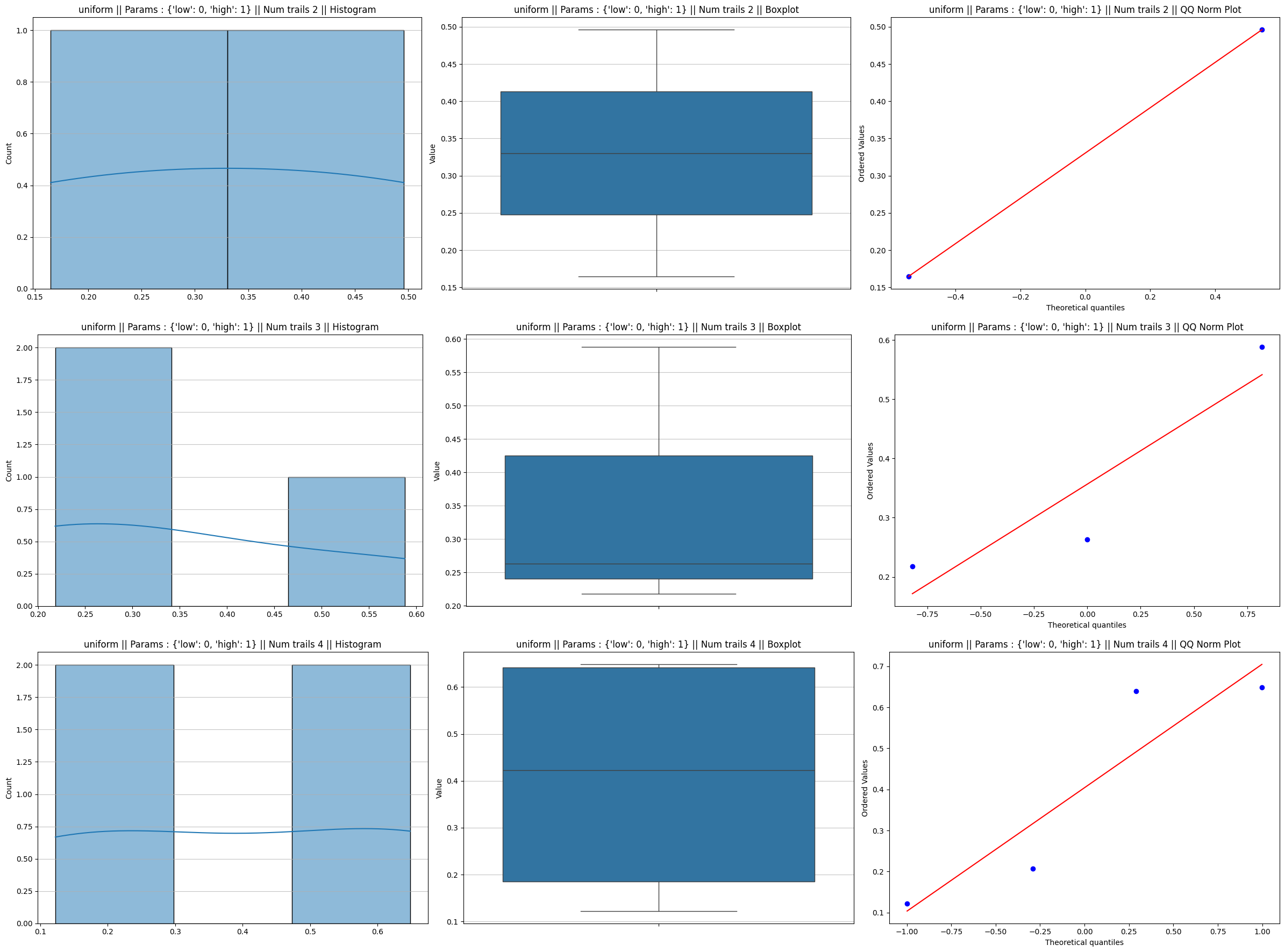
Uniform distribution

Uniform distribution achieves normality quite faster compared to other distribution even with trails as low as 5.

The speed of convergence to a Normal distribution is primarily dictated by two factors: Symmetry and Tails

Perfect Symmetry: Unlike the Binomial (with $p \neq 0.5$) or the Exponential distribution, the Uniform distribution is perfectly symmetric around its mean ($\mu = \frac{a+b}{2}$). Because there is no “skew” to correct, the CLT doesn’t have to work as hard to balance the distribution
Lack of Outliers (No Heavy Tails): The Uniform distribution is strictly bounded between $a$ and $b$. There are no extreme values or long “tails” that could pull the sample mean far away from the center
The “Irwin-Hall” Effect: The sum of independent uniform variables actually has its own named distribution called the Irwin-Hall distribution. By the time you sum just 3 uniforms, the resulting shape is already a smooth curve (though slightly flat at the top). By $n=5$, the density function is mathematically almost indistinguishable from a Gaussian bell curve

This proves that “sufficiently large $n$” is not a fixed number—it is a variable that depends entirely on how much the starting distribution “disagrees” with the symmetry of a Normal curve.

Uniform distribution plots

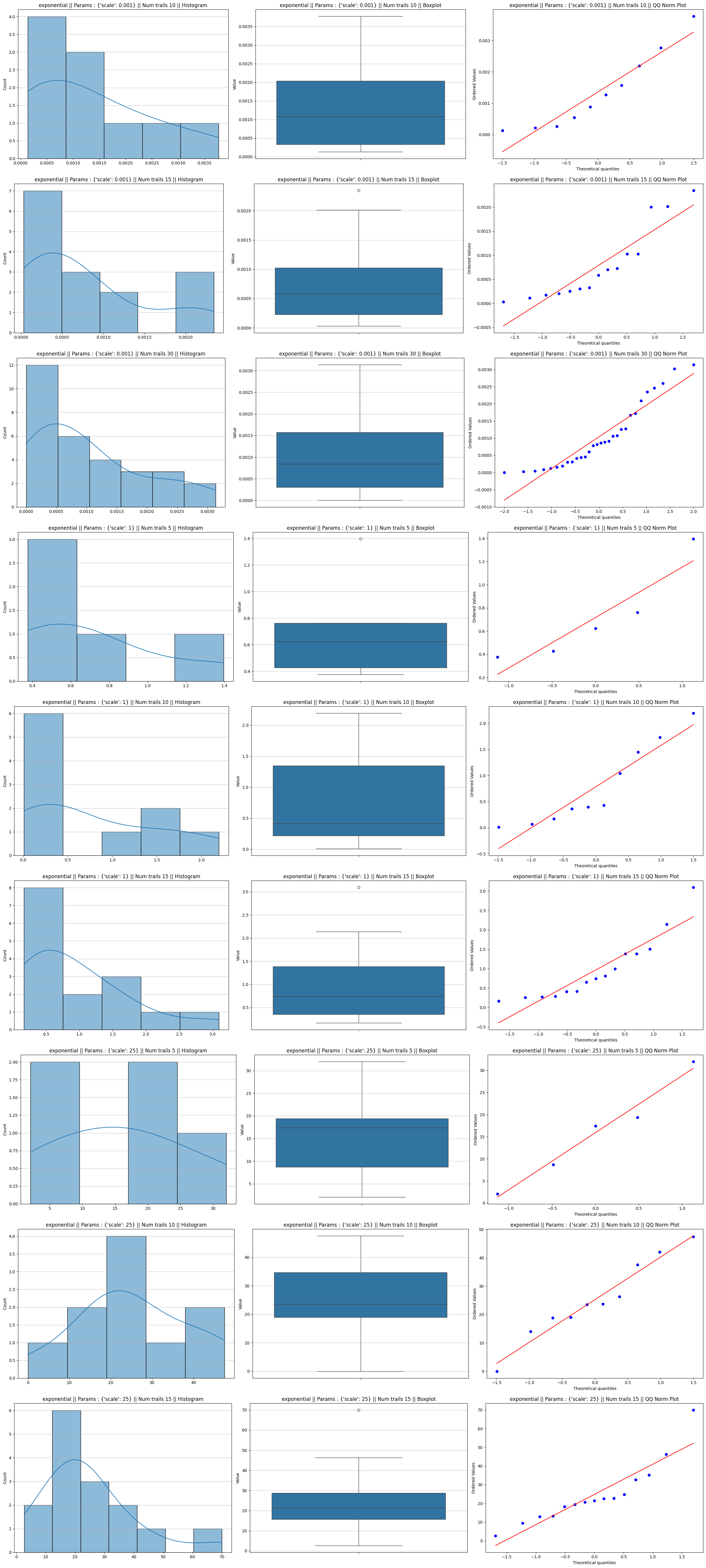
Exponential distribution

Normality is achieved ONLY by increasing the sample size $n$. Whether $\lambda = 0.001$ or $\lambda = 25$, an individual exponential observation is always highly skewed. You will always need a solid sample size (typically 1$n \ge 30$) to see a normal distribution in the sample means

Exponential distribution plots

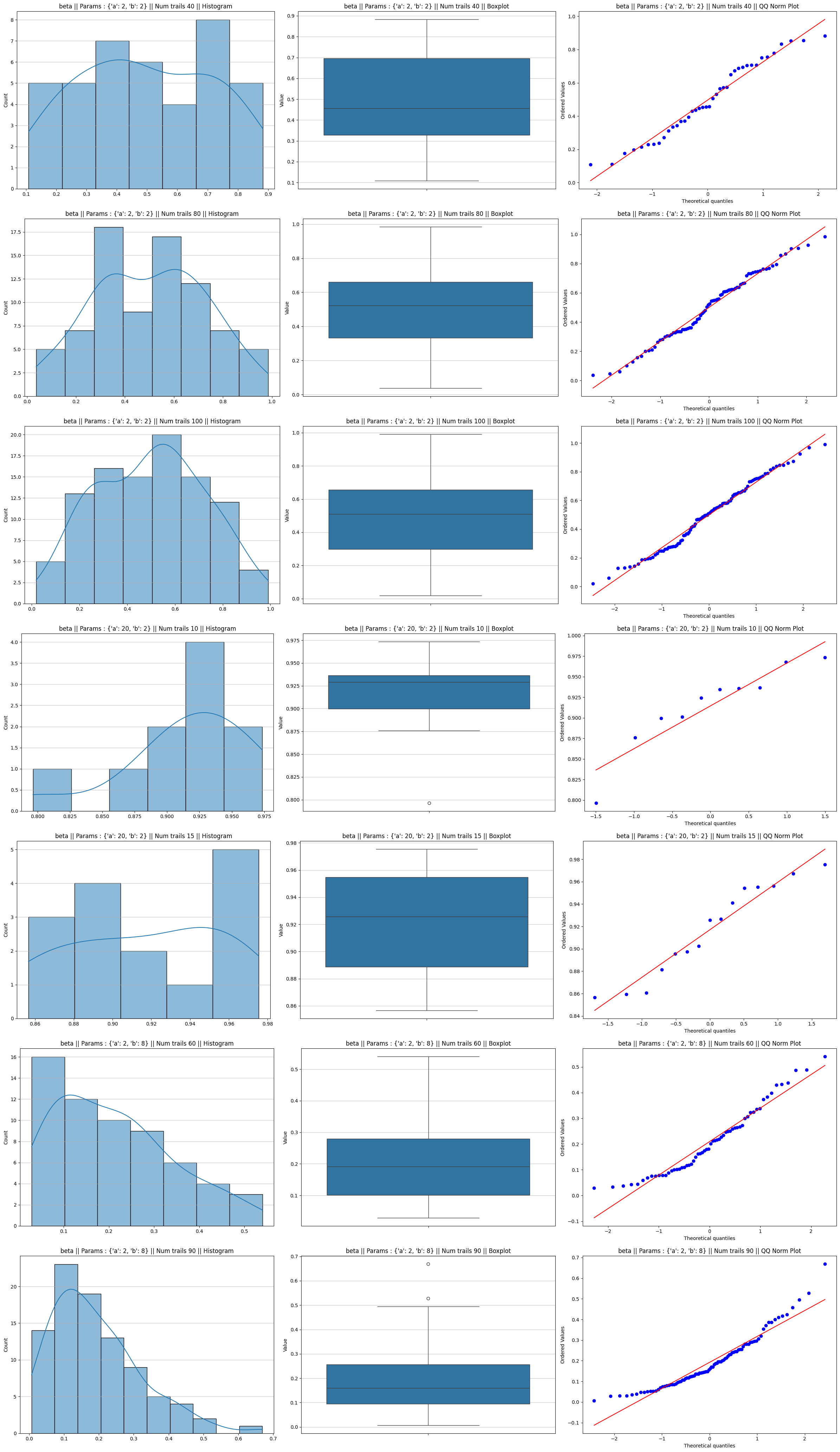
Beta distribution

The Beta distribution is unique because it is defined on the interval $[0, 1]$ and its shape can change drastically based on its parameters:

When $\alpha = \beta$: The distribution is perfectly symmetric
- If $\alpha = \beta = 1$, it is a Uniform distribution (which, as you noted earlier, converges extremely fast, around $n=5$)- If $\alpha = \beta = 3$, it looks like a “hump” that is already quite close to a Normal shape. Normality is achieved almost immediately
When $\alpha \neq \beta$: The distribution becomes skewed
- If $\alpha < \beta$, the distribution is “pushed” to the left (Right-skewed)
- If $\alpha > \beta$, the distribution is “pushed” to the right (Left-skewed)

Beta distribution plots

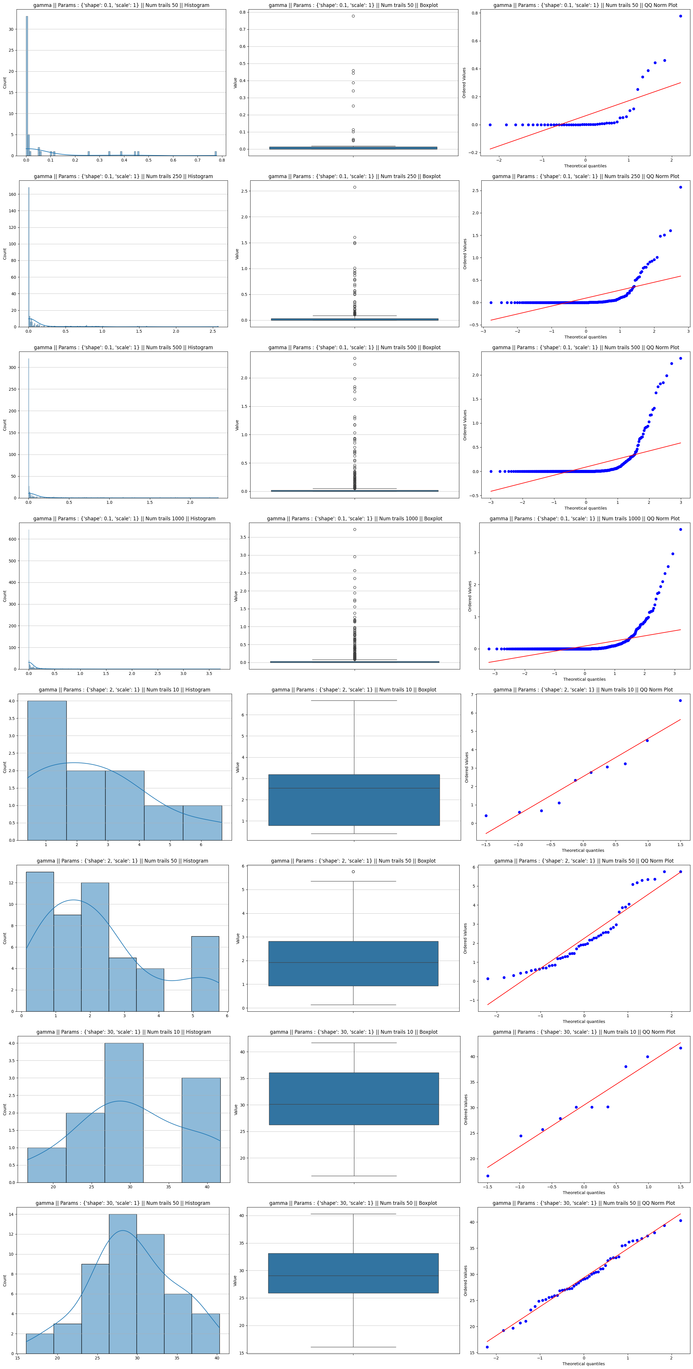
Gamma distribution

The Gamma distribution’s shape is controlled by the shape parameter ($k$). The skewness of a Gamma distribution is defined as $2/\sqrt{k}$.

The “Resistant” Case: Shape = 0.1 When your shape parameter is 0.1, the skewness is roughly 6.32. This is an incredibly “sharp” distribution, where almost all values are clustered near zero, with a very long, thin tail.
- Even at $n=1000$, it is “Not normal
- “Why: The “mass” of the distribution is so heavily concentrated at one extreme that even averaging 1,000 samples isn’t enough to pull the mean away from the boundary and create the symmetric right-hand tail needed for a Gaussian curve. For a shape of 0.1, you might need $n > 5000$ to finally pass a normality test
The “Fast” Case: Shape = 2 and Shape = 30
- Shape = 2: The skewness drops to 1.41. Because the “starting point” is much less distorted, your test shows it becomes “normally distributed” with a sample size as low as $n=10$
- Shape = 30: The skewness is only 0.36. At this point, the Gamma distribution already looks like a bell curve before you even apply the CLT. That is why your p-values (0.86 and 0.67) are so high—the data is “born” almost normal.

Gamma distribution plots

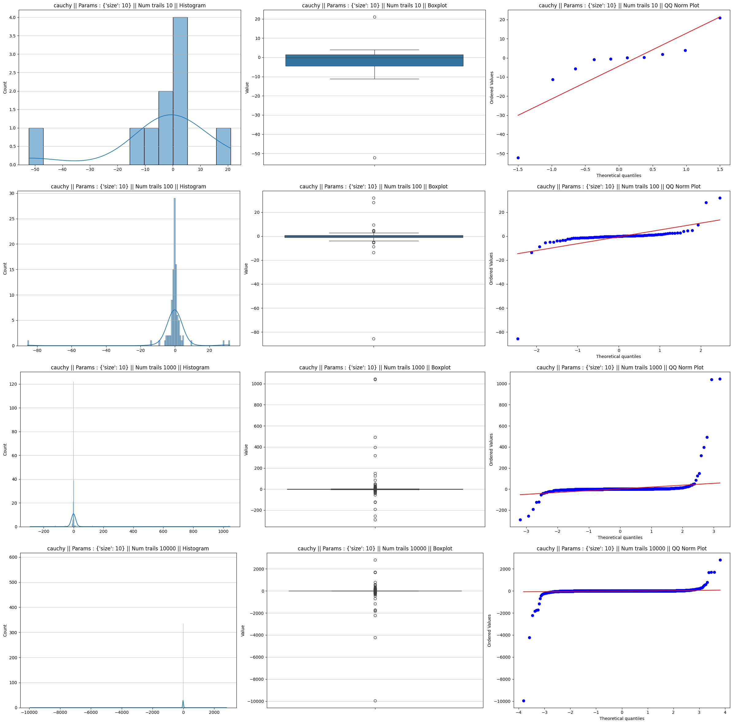
Cauchy distribution

The Cauchy distribution has “Fat Tails” so extreme that the mean and variance are mathematically undefined. If you take the average of 1,000 Cauchy samples, the result is still a Cauchy distribution. It never “thins out” into a Normal tail.

Cauchy distribution plots

P Value table comparison using both the test

Further Qualitative observations

Summary of observations

Distribution	Convergence Speed	Why? (The Simple Reason)
Uniform	Ultra-Fast ($n \approx 5$)	It is perfectly symmetric and has no outliers; it’s already halfway to a bell curve.
Normal	Instant ($n=1$)	It is already normal! Sampling doesn’t change the shape, only the spread.
Beta	Fast (if $\alpha \approx \beta$)	When parameters are equal, it is symmetric. “Unbalanced” parameters create skew.
Binomial	Moderate (at $p=0.5$)	Symmetric but “chunky” (discrete). It needs some to fill the gaps between bars.
Gamma	Variable	Low shape parameters () create a “spike” that is very hard for the CLT to smooth out.
Exponential	Moderate/Slow	It is always one-sided (skewed). It always needs to build the “missing” left tail.
Poisson	Slow (for low $\lambda$)	At low , it’s mostly zeros. You need huge samples to find enough “events” to balance it.
Cauchy	Never	It has “infinite variance.” The outliers are so extreme they break the math of the CLT.

The Outlier: Why the Cauchy Distribution Fails

During the analysis, one would have likely noticed that the Cauchy distribution refused to conform to the bell curve, no matter how large the sample size became.

This happens because the CLT has a strict prerequisite: the population must have a finite mean and finite variance. The Cauchy distribution is “pathological”—its tails are so heavy that the integral used to calculate the mean does not converge. In mathematical terms, its variance is undefined.

Because the “average” of a Cauchy sample is dominated by extreme outliers that do not diminish with larger , the sample mean remains as volatile as a single observation. It follows a Cauchy distribution regardless of , effectively “breaking” the Central Limit Theorem.

Conclusion and Scope for Further Exploration

Our empirical analysis confirms that for most distributions, the CLT is remarkably robust. Even highly skewed distributions like the Exponential or Gamma eventually yield a beautiful bell curve for the sample mean once .

Further Scope for Exploration:

Rate of Convergence: Investigate how the “Skewness” of the initial distribution affects the required to reach normality (e.g., does a highly skewed Beta distribution require vs ?).
The Lindeberg-Feller Condition: Explore cases where the random variables being averaged are not identically distributed (Non-IID).
Multivariate CLT: Extend this analysis to vectors and higher-dimensional data spaces.

statistics

This post is licensed under CC BY 4.0 by the author.