On Policy VS Off Policy
Introduction
While learning basics of RL , Many would ponder over the question of what is the difference between a off policy learning strategy vs a on policy learning strategy. Many learners, in a hurry, would assume its essentially learning startegy based on the method of deployment “Online” vs “Offline”. However the truth is far from that. Also a few would assume, there is no difference between both the technqiue and would lead to the same final policy in terms of picking the best action, While this could be true in some cases, it is not true for many environments.
In this blog, we will try to see the difference between them with an example startegy from each paradigm and will try them on the same environment. We will be using CliffWalking-v1 environment for demonstrating Q-Learning and SARSA.
In theory what is the difference between On Policy and Off Policy learning
The textbook definition of On Policy learning states that the agent learns directly from the actions taken by the current policy, While Off Policy learning has 2 different policies: A behaviour policy that generates actions and a target policy that is trained using the data.
To understand them in detail, we have to see the update rules of the examples we have picked.
- SARSA [ On Policy ]
For SARSA (on-policy learning), the Q-value is updated using the current state-action pair and the next state-action pair sampled from the same policy:
\[\begin{equation} Q(s_t, a_t) \leftarrow Q(s_t, a_t) + \alpha \left[ r_{t+1} + \gamma Q(s_{t+1}, a_{t+1}) - Q(s_t, a_t) \right] \end{equation}\]Where:
- $ Q(s_t, a_t) $ is the current estimate of the Q-value for state $s_t$ and action $a_t$.
- $ \alpha $ is the learning rate.
- $ r_{t+1} $ is the reward received after taking action $a_t$ in state $s_t$.
- $ \gamma $ is the discount factor.
- $ Q(s_{t+1}, a_{t+1}) $ is the Q-value for the next state $s_{t+1}$ and the next action $a_{t+1}$ chosen by the same policy.
- Q-Learning [ Off Policy ]
For Q-learning (off-policy learning), the update uses the maximum Q-value over all possible actions in the next state, regardless of the policy:
\[\begin{equation} Q(s_t, a_t) \leftarrow Q(s_t, a_t) + \alpha \left[ r_{t+1} + \gamma \max_{a} Q(s_{t+1}, a) - Q(s_t, a_t) \right] \end{equation}\]Where:
- $\max_{a} Q(s_{t+1}, a)$ represents the maximum Q-value among all possible actions in the next state $s_{t+1}$.
The key difference between the above 2 updates rules is in the choice of next action. SARSA picks the next action based on the same policy (current policy) is becomes an example of a On policy learning method. Q learning assumes the next possible action is chosen based on the highest Q value (greedy approach), which makes it a off policy learning.
What difference does it make ?
This key difference allows the Off policy methods to learn from experiences generated by different (older and other explorative) policies or even from collected data. The usage of 2 different policies (behaviour vs target) essentially decouples the data collection based on multiples policy and learning a target policy. This decoupling makes off-policy methods more flexible and potentially more sample efficient.
Lets see it with an example. Below are the support functions and classes for running a SARSA and Q-learning in a cliff walking environmnt.
Function to plot the heatmap of the policy with direction chosen by the agent.
1
2
3
4
5
6
7
8
9
10
11
12
13
14
15
16
17
18
19
20
21
22
23
24
25
26
27
28
29
30
31
32
33
34
35
36
37
38
39
40
41
42
43
44
45
46
47
48
49
50
51
import numpy as np
import gymnasium as gym
import imageio
import time

def plot_heatmap(Q):
    # Extract the max Q-value for each state
    state_values = np.max(Q, axis=1)

    # CliffWalking is a 4x12 grid
    height, width = 4, 12

    # Reshape state values into grid layout for visualization
    state_values_grid = state_values.reshape((height, width))

    # Plot heatmap with annotations
    plt.figure(figsize=(12, 4))
    plt.title("CliffWalking State Values Heatmap with Values and Policy Arrows")
    im = plt.imshow(state_values_grid, cmap='viridis', interpolation='nearest')
    plt.colorbar(im, label='Max Q value')
    plt.xticks(np.arange(width))
    plt.yticks(np.arange(height))
    plt.gca().invert_yaxis()

    # Action to arrow direction mapping for CliffWalking actions
    # Assuming actions: 0=UP, 1=RIGHT, 2=DOWN, 3=LEFT
    arrow_dict = {
        0: (0, -0.3),  # Up: arrow goes up (negative y)
        1: (0.3, 0),   # Right
        2: (0, 0.3),   # Down
        3: (-0.3, 0)   # Left
    }

    for i in range(height):
        for j in range(width):
            # Text annotation of max Q value
            plt.text(j, i, f"{state_values_grid[i, j]:.2f}",
                     ha='center', va='center',
                     color='white' if state_values_grid[i, j] < (state_values_grid.max() / 2) else 'black')

            # Get best action for state
            state_index = i * width + j
            best_action = np.argmax(Q[state_index])

            # Arrow displacement
            dx, dy = arrow_dict[best_action]

            # Draw arrow with red color
            plt.arrow(j, i, dx, -dy, color='red', head_width=0.15, head_length=0.15)

    plt.show()
Function to render the environment
1
2
3
4
5
6
7
8
9
10
11
12
13
14
15
16
17
18
19
20
21
22
23
24
25
26
27
28
29
30
31

def render_env(Q):
    env = gym.make('CliffWalking-v1', render_mode='rgb_array')

    # Assuming you have a trained Q-table called Q
    # Q = np.random.rand(env.observation_space.n, env.action_space.n)  # Replace with trained Q-table

    frames = []

    state, _ = env.reset()
    done = False
    total_reward = 0

    while not done:
        frame = env.render()  # returns RGB numpy array
        frames.append(frame)

        action = np.argmax(Q[state])
        state, reward, done, _, _ = env.step(action)
        total_reward += reward

    # Append final frame
    frames.append(env.render())

    env.close()

    # Save frames as GIF
    gif_filename = 'cliffwalking_agent.gif'
    imageio.mimsave(gif_filename, frames, fps=4)  # Adjust fps as needed

    print(f"Saved GIF as {gif_filename}")
An Agent classes with 2 choices of startegy.
1
2
3
4
5
6
7
8
9
10
11
12
13
14
15
16
17
18
19
20
21
22
23
24
25
26
27
28
29
30
31
32
33
34
35
36
37
38
39
40
41
42
43
44
45
46
47
48
49
50
51
52
53
54
55
56
57
58
59

# Hyperparameters
ALPHA = 0.1       # learning rate
GAMMA = 0.99      # discount factor
EPSILON = 0.1     # exploration probability
EPISODES = 10000   # number of episodes
MAX_STEPS = 100   # max steps per episode

class agent:

    def __init__(self):
        self.env = gym.make('CliffWalking-v1')
        n_states = self.env.observation_space.n
        n_actions = self.env.action_space.n
        self.Q = np.zeros((n_states, n_actions))

    def epsilon_greedy_action(self, state):
        if np.random.rand() < EPSILON:
            return self.env.action_space.sample()
        return np.argmax(self.Q[state])

    def train(self, strategy="Q"):
        # Q-learning algorithm
        for ep in range(EPISODES):
            state, _ = self.env.reset()
            done = False
            for _ in range(MAX_STEPS):
                action = self.epsilon_greedy_action(state)
                next_state, reward, done, truncated, _ = self.env.step(action)

                # Q-learning update rule
                if strategy=="Q":
                best_next_action = np.argmax(self.Q[next_state])
                self.Q[state, action] += ALPHA * (reward + GAMMA * self.Q[next_state, best_next_action] - self.Q[state, action])
                elif strategy=="SARSA":
                next_action = self.epsilon_greedy_action(next_state)
                self.Q[state, action] += ALPHA * (reward + GAMMA *self.Q[next_state, next_action] - self.Q[state, action])
                else:
                raise ValueError("Invalid strategy. Choose 'Q' or 'SARSA'.")

                state = next_state
                if done or truncated:
                    break

        return self.Q

    def evaluate(self):
        state, _ = self.env.reset()
        done = False
        total_reward = 0

        while not done:
            action = np.argmax(self.Q[state])
            state, reward, done, _, _ = self.env.step(action)
            total_reward += reward

        print("Total reward following learned policy:", total_reward)
        return total_reward
Finally execution and evaluation of the agent.
1
2
3
4
5
6
7
rl_agent = agent()
Q_table = rl_agent.train()
rl_agent.evaluate()

rl_agent = agent()
sarsa_table = rl_agent.train(strategy="SARSA")
rl_agent.evaluate()
One would notice the total reward of Q learning agent is always greater than the total reward of SARSA agent. This is not a random mistake, Even running the same simulation multiple times will show you that the total rewards status remains unchanged.
It is always that the SARSA agents takes more steps while the Q learning agents takes few lesser steps to achieve the same result.
Below is the visualisation of the environment and path taken by both the agent.
1
2
render_env(q_table)
render_env(sarsa_table)

Does that mean Q learning is better ? No, the answer is clear in the q table
1
2
plot_heatmap(q_table)
plot_heatmap(sarsa_table)
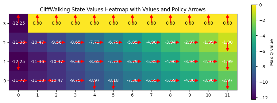
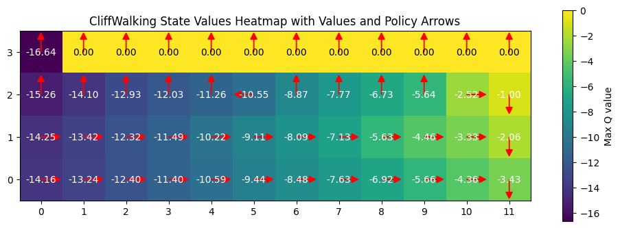
From the table, it is clear that the q learning algorithm takes a much more riskier route (closer to the cliff) compared to the SARSA algorithm takes a safer route. This also highlights how greedy policy can compromise a quality output and risking the end goal, while onpolicy even takes a bit longer but has a better chance of reaching the end goal. **The q learning agent can thus converge to suboptimal policies if the exploration is insufficient or even if the reward is biased. **
Key difference between On-Policy and Off-Policy learning
| Aspect | On-Policy RL | Off-Policy RL |
|---|---|---|
| Data source | Data generated by the current policy | Data can be from different policies |
| Policy updates | Same policy for behavior and learning | Separate behavior and target policies |
| Examples | SARSA | Q-learning |
| Sample efficiency | Lower, as learning is tied to current policy exploration | Higher, through reuse of varied data |
| Stability | Generally more stable and predictable | Potentially less stable but more flexible |
| Complexity | Simpler algorithms and tuning | More complex with convergence challenges |
| Optimality | Risks local optima due to policy coupling | Better at finding global optimum solutions |
Overall, Both approaches have merits and its has become common in modern RL to combine principles from both the strategies to yield better results. ( Actor critic - DDPG algorithm )